Computing Science: the study of how to solve problems efficiently
(It's not engineering, not technology --- It's science: the application of
methodology and experimentation to obtain knowledge of a phenomenom.)
- Solvability: computability theory
- Efficiency: computational complexity theory
Modern computing technology is a consequence of computing science....
Solvability: Computability theory
In the 19th century, mathematicians were the computers; they
computed with deduction laws. They computed proofs.
Have you taken a Geometry class? If so, you computed the
classical way.
A tiny example: deduction laws for "less-than":
===================================================

         E1 > E2                              E1 > E2    E2 > E3
(add):------------------    (transitivity): -----------------------
       E1 + N > E2 + N                             E1 > E3

===================================================
Two proofs using these laws:
===================================================

PROVE: |-  x + 2 > x                   PROVE: a > 0, a > b |-  a + a > b

1.   2 > 0          arithmetic fact    1.  a > 0          hypothesis
2.   x + 2 > x + 0  add 1              2.  a > b          hypothesis
3.   x + 2 > x      arithmetic on 2    3.  a + a > a + 0  add 1
                                       4.  a + 0 > b + 0  add 2
                                       5.  a + a > b + 0  transitivity 3,4
                                       6.  a + a > b      arithmetic on 5

===================================================
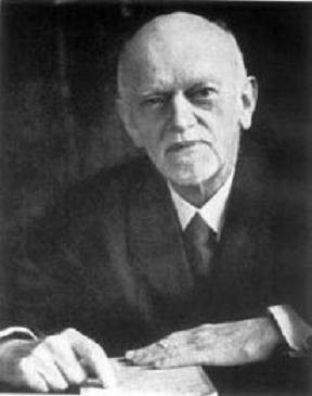
Hilbert's Program
|
David Hilbert was perhaps the most influential mathematician
of the 19th (and 20th!) centuries. Hilbert believed strongly in the
computing approach to mathematics, like above, and in the 1920's he
employed many mathematicians to realize "Hilbert's program":
all true facts of mathematics can be computed by proofs using
deduction laws for classical logic ("and", "or", "not", "all",
"exists") and numbers (like the two laws above).
This implies that all of mathematics can be done (by machines!)
that mechanically apply deduction laws in all possible combinations until
all true facts are computed as answers.
Will this work out? Are humans unnecessary to mathematics?
|
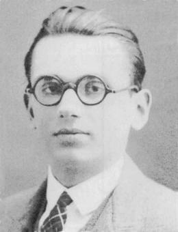
Gödel's Incompleteness Proof: "The most important result of the 20th century" and the beginning of modern computing science
|
In 1931, a German PhD student, Kurt Gödel ("Goedel"), showed that Hilbert's program
was impossible --- he showed that mathematics was unsolvable ---
there are true facts in math that cannot be computed mechanically.
In the process, Gödel invented the modern notions of
machine coding, stored program, recursive computation, and program analyzer (a program that consumes other programs as inputs).
|
Greatly simplified, here's what Gödel did:
-
He invented machine coding (like ASCII coding): he represented symbols
like x, >, and 2, as numbers (in ASCII, these would be
#120, #062, #050) so that a mathematics formula like x > 2 is machine-coded
as 120,062,050 --- one long number.
-
He machine-coded deduction laws and multi-line proofs
as huge numbers, just like .exe-files are huge numbers.
-
He showed how to write computer programs, as formulas in
classical logic (using true-false predicates, "and", "or", "not", "all", "exists") in
a programming-language style
he invented, called primitive-recursive functions.
He wrote programs (logic formulas) that (i) check if a number
decodes into a formula; (ii) check is a number decodes into a proof;
(iii) check if a numbered proof proves a numbered formula.
He explained how to generate mechanically
all combinations of all deduction laws to
prove all the facts of mathematics that can be proved.
The big question is: Will the deduction laws prove all the
true facts of mathematics or just some of them?
That is, is Hilbert's program possible?
Gödel studied the deduction laws for
schoolboy (Peano)
arithmetic: the nonnegative ints with +, *, >, =, and
he proved there are true facts of arithmetic that can never be proved by
deduction laws!
Gödel did this by finding a formula, which has
integer number, #G, such that:
-
#G = Formula #G cannot be proved
Formula #G says, ''I cannot be proved!''
(More precisely stated, ``Formula #G cannot be proved'' is this logic formula:
¬(∃ P (decodesIntoProof(P) ∧ decodesIntoFormula(#G) ∧ proves(P, #G))), that is,
``There does not exist an int, P, that decodes into a proof of the formula numbered by int G.'')
-
Gödel constructed Formula #G as a consequence of his amazing
recursion theorem --- for any logic system that can express
arithmetic, conditional choice, formulas-as-ints, and staging,
-
for this pattern, Formula #___ cannot be proved,
-
there must be an integer, call it G, such that Formula #G has exactly
the same true-false meaning as (is logically equivalent to) the formula, Formula #G cannot be proved.
Assume that the deduction laws (i) build proofs of only true formulas
(the laws are sound) and (ii) can build proofs for all the true formulas of arithmetic (the laws are complete).
Can the deduction laws for arithmetic be both sound and complete?
Assume they are.
Formula #G is a logical bomb that blows up our assumption:
-
#G = Formula #G cannot be proved
-
If Formula #G is true, then the complete deduction laws build a proof of Formula #G. But since Formula #G is true, then so is Formula #G cannot be proved.
But the complete deduction laws have proved Formula #G! This is a contradiction --- it's impossible.
-
If Formula #G is false, then the sound deduction laws clearly cannot prove it.
But the falsity of Formula #G says that not(Formula #G cannot be proved) is true, which means that the deduction laws must prove Formula #G! This is also a contradiction --- impossible.
The only way to escape both contradictions is to conclude that
Formula #G is a true fact of arithmetic and no sound
set of deduction laws can ever prove it:
-
Any set of sound deduction laws for arithmetic must be incomplete.
Side comment: It's not odd that logic formulas can code computation --- this has been known for centuries. Gödel was the first to make a computer language out of logic, and these days, the PROLOG ("PROgramming in
LOGic") programming language is the preferred language for
artificial intelligence, knowledge discovery, and even some data-base applications.
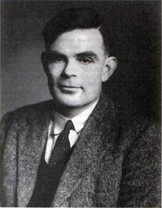
Turing machines and von Neumann machines
Gödel's work shattered Hilbert's program and it generated an intensive
study of what machines might and might not be capable of solving.
One person who took interest was Alan Turing.
|
Turing was an English mathematician, employed by the British government to break the codes the Nazi armies used for communication. Turing and his team succeeded, and the Allies used the decoded Nazi communications to win World War II.
Turing was interested in mathematical games, and he was interested in the machine codings of Gödel. He conceived a machine for working with the codes. His Turing machine was a controller with a read-write head that traversed the squares of an unbounded roll of toilet paper, where only a 0
or a 1 can be written in a square:
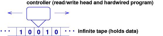
|
Turing realized that the controller could be wired
as a "processor" that understood this instruction set:
move Left/Right one square
erase the square (make it blank)
write 0/1 on the square
if square is blank/0/1, then goto Instruction #n
goto Instruction #n
stop
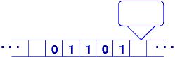
Here is a sample program that scans a binary number from left to right and flips all 0s to 1s and all 1s to 0s:
#1: if square is 0, then goto #4
#2: if square is 1, then goto #6
#3: if square is blank, then goto #9
#4: write 1
#5: goto #7
#6: write 0
#7: move Right
#8: goto #1
#9: stop

             ... => ...
These instructions are given number codings, so that a program written in the
instructions could be copied on a tape and read by a controller.
The Universal Turing Machine was configured like this:
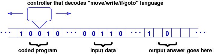
Gödel's machine codings were used to represent a program as a long sequence of 0s and 1s. The Universal Turing Machine is the origin of
-
CPU
-
linear storage
-
stored program
-
binary machine language
Turing wrote programs for the Universal Turing machine, and all the programs
of Gödel's primitive-recursive-function language were coded for the Turing
machine. Turing believed that all facts/knowledge/problems that can be calculated/deduced/solved by a machine can be done by a Universal Turing Machine.
This is now known as the Church-Turing thesis.
(The "Church" part refers to Alonzo Church, a Princeton mathematician
who developed a symbol system, the lambda-calculus, which has the same
computational powers as Turing's machines.)
Turing asked: are there some problems whose solutions cannot be calculated by his machine?
Here is the problem he considered: It is the first example of a
program analyzer:
Is there a program that can read the machine coding of any other program
and correctly predict whether the latter will loop when it runs?
This is called the halting problem.
Turing showed that the answer is NO --- there is
no such program. Here's why:
-
If such a program, H, existed, it would have a machine coding, say, #H,
and it would have to behave like this:
H(#P) = print 0, if  program #P loops when it runs
        print 1, if  program #P halts when it runs
(If Program #P itself needs input data, the input data number is appended on the tape to the end of int #P.)
-
We use program #H to build this ``evil-twin program'', E:
E(#P) = start program #H with #P on the same tape as input.
        Wait for the answer.
        If the answer's 1, then  LOOP!
        If the answer's 0, then print 0
-
Now, what is the outcome of running program E with its own coding, #E?
E(#E) loops exactly when H(#E) prints 1, that is, when E halts!
And, if E(#E) halts, printing 0, it is exactly because E loops!
Both cases are impossible --- program H cannot exist, because it would
let us build evil-twin program E and generate the logical impossibility that follows.
The halting problem specifies a problem that can never be solved by a machine.
As a consequence,
many other program-analysis problems are readily proved impossible to
implement:
-
whether a program is free of all run-time errors
-
whether two programs produce exactly the same outputs from the same inputs
-
whether a program matches a logical requirement of correctness behavior.
None of these problems are solvable in the general case, but
computer scientists have identified subcases of the above
problems and have developed programs/tools/logics that can do useful
program analysis. This is what I do for my paychecks (in addition
to teaching, doing paperwork and administration, etc.).
Von Neumann machines
Modern computers use architectures based on
Universal Turing Machines. The adaptation is due to Eckart, Mauchley and von Neumann,
at the University
of Pennsylvania, where they built the ENIAC electronic computer:
The first electronic computers were "non universal" machines, where
the computer program was wired into the CPU. The wires were moved around
when a new program was desired. The ENIAC people implemented
Gödel's and Turing's machine language, stored programs, and "universal" CPUs.
Your computers and electronic gadgets are the offspring of Gödel's and Turing's thoughts.
The developments described here crystallized as computability theory.
Classes of solvable problems
Gödel and Turing showed that many critical math and programming problems
will never be solved by machine. But many can be, and the classes of solvable
problems have been intensively studied.
First, think of a problem as a math function: you give
an input argument to the function, and the function tells you an answer (output).
The function defines what you must solve/implement.
Now, which math functions can be mechanically computed
by programs? Here are two famous groups that can:
-
the primitive-recursive functions (Gödel): These are
functions on numerical inputs that are computed by
0, +1, calling other primitive-recursive functions, and self-call
(recursion). This class of functions includes most of arithmetic, and
their programs always halt --- an input will always produce an output.
-
the μ-recursive functions (S.C. Kleene): These are
functions on numerical inputs that are computed by
0, +1, calling other μ-recursive functions, self-call,
and minimalization (``find the least nonnegative int such that...'').
This class of functions matches exactly the functions computed by programs
written for Turing machines. The programs are not guaranteed to halt.
Within these two groups lie many subclasses: (i) within the
primitive-recursive functions lies the Grzegorczyk hierarchy of solvability;
(ii) within the μ-recursive functions lies the modern time-complexity
hierarchy; see the next section.
Efficiency: Computational Complexity Theory
Say that a problem can be solved by a computer (that is, it is one of
the μ-recursive functions) --- how good is the solution
(program)? How fast? How much storage space
is needed? Is the solution the best possible for solving the problem?
These questions are studied within computational complexity theory.
Their answers define subclasses of the μ-recursive functions.
We learn about this topic by studying
some simple algorithms that work with arrays.
Linear-time algorithms
Say you have a database that is an array of int keys connected to data records. The keys aren't arranged in any special way, so finding
a data record by its key requires a linear search of
an array of ints, e.g.,
find key 8 in array, [6, 10, 2, 4, 12, 16, 8, 14]:
Step 1:  V
        [6, 10, 2, 4, 12, 16, 8, 14]

Step 2:      V
        [6, 10, 2, 4, 12, 16, 8, 14]
...

Step 7:                       V
        [6, 10, 2, 4, 12, 16, 8, 14]
We search the array from front to back. How fast is this algorithm?
Without worrying about speeds of chips, we measure the speed of an
array algorithm by how many array lookups/updates it must do.
Obviously, with an array of length 8, at most 8 lookups is needed;
in general, if the array has length N, at most N lookups is needed.
This is the worst-cast time complexity, and in this case is
linearly proportional to the length of the array. We say that sequential
search is a linear-time algorithm, order-N.
Here is a table of how a linear-time algorithm performs:
===================================================

array size, N        worst-case time complexity, in terms of lookups
----------------------------------------------
64                   64
512                  512
10,000               10,000

===================================================
A linear-time algorithm looks "slow" to its user but is tolerable if
the data structure is not "too large".
When you write a one-loop program that counts through the elements of
an array, your algorithm runs in linear time.
Log-time algorithms
What if the array of keys was sorted so that the keys were in ascending
order?
In this case, we can use a "dictionary lookup" algorithm, called
binary search, which jumps into the middle of the array,
looks at the key there, and then jumps into the middle of the left half or
right half, depending whether the desired key is less-than or greater-than the
key in the middle:
Find 8 in  [2, 4, 6, 8, 10, 12, 14, 16, 18, 20, 22]:

Step 1: look in middle:     V
           [2, 4, 6, 8, 10, 12, 14, 16, 18, 20, 22]

Step 2: look in middle of left half:     V
                                  [2, 4, 6, 8, 10 ... ]

Step 3: look in middle of left's right subhalf:    V
                                            [ ..., 8, 10, ... ]
The subarray searched shrinks by half each time there is a
lookup, and the key is quickly found --- in worst case,
at most log2N lookups are needed to find the key. (Recall that
log2N = M means that 2M = N.)
This is log-time, order log-N.
Here's a table:
===================================================

array size, N   linear-time  log-time
----------------------------------------------
64               64          6
512              512         8
10,000           10,000      12

===================================================
The speed-up is spectacular; this algorithm is markedly faster in
theory and in practice. In practice, regardless of how a database
is configured, the search operation must be order log-time or faster.
When you write an algorithm that "discards" half of a data structure
during each processing step, you are writing a log-time algorithm.
Quadratic-time algorithms
How much time does it take to sort an array of keys into ascending order?
A standard technique, called selection sort, works like this:
Input array                     Output array
---------------------------    --------------------
[6, 10, 2, 4, 12, 16, 8, 14]    []

[6, 10, 4, 12, 16, 8, 14]       [2]

[6, 10, 12, 16, 8, 14]          [2, 4]

[10, 12, 16, 8, 14]             [2, 4, 6]

 . . .

[16]                            [2, 4, 6, 8, 10, 12, 14]

[]                              [2, 4, 6, 8, 10, 12, 14, 16]
The algorithm scans the N-element array N-1 times, and
1/2(N2 - N) lookups are done; there are also N updates to the
output array. This is a quadratic-time algorithm, order N2. Here is the comparison table:
===================================================

array size, N   linear     log2N   N2          1/2(N2 + N)
-------------------------------------------------------
64               64        6     4096         2064
512              512       8     262,144      131,200
10,000           10,000    12    100,000,000  50,002,500

===================================================
(Note there isn't a gross difference between the numbers in the last two columns. That's why selection sort is called a quadratic-time algorithm.)
A quadratic-time algorithm runs slowly for even small data structures.
It cannot be used for any interactive system --- you run this kind
of algorithm while you go to lunch.
When you write a loop-in-a-loop to process
an array, you are writing a quadratic algorithm.
The standard sorting algorithms are quadratic-time, but there is a clever
version of sorting, called "quicksort", that is based on a
divide-and-conquer strategy, using a kind of binary search to replace one
of the nested loops in the standard sorting algorithms. Quicksort runs in order N * log2N time:
N      log2N     N2          N*log2N
-------------------------------------------------------
64     6       4096         384
512    8       262,144      4096
10,000 12      100,000,000  120,000
===================================================
Intractable problems and their algorithms
Say you have a maze, and you want to calculate the shortest path of all the
paths from
the maze's entry to its exit. Or say you have a deck of cards,
and you want to print all the shuffles of the deck. Or you have a roadmap
of cities, and you want to calculate the shortest tour that lets you visit
each city (this is the travelling salesman problem):
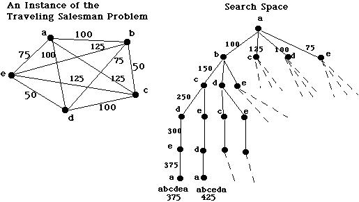
These problems require that you calculate all possible permutations (internal combinations) of
a data structure before you select the best permutation.
Many important industrial and scientific problems, which ask for optimal
solutions to complex constraints, are minor variations of the
search-problems stated here.
The problems stated above are solvable --- indeed,
here is a Python function that calculates all the permutations (shuffles) of a deck of
size-many cards:
===================================================

def permutations(size) :
    """computes a list of all permutations of [1,2,..upto..,size]
       param: size, a nonnegative int
       returns:  answer, a list of all the permutations defined above
    """
    assert size >= 0
    if size == 0 :
        answer = [[]]  # there is only the "empty permutation" of a size-0 deck
    else :
        sublist = permutations(size - 1)  # compute perms of [1,..upto..,size-1]
        answer = []   # build the answer for  size-many  cards in a deck
        for perm in sublist:
            # insert  size  in all possible positions of each  perm:
            for i in range(len(perm)+1) :
                answer.append( perm[:i] + [size] + perm[i:] )
    return answer

===================================================
It uses a recursion and a nested loop. For example,
permutations(3) computes
[[3, 2, 1], [2, 3, 1], [2, 1, 3], [3, 1, 2], [1, 3, 2], [1, 2, 3]].
Try this function on your computer and see how large an argument you
can supply until the computer refuses to respond.
The solution to the above is written in just a few lines of Prolog, which is
an ideal language for calculating all combinations that satisfy a set
of constraints:
===================================================

/* permutation(Xs, Zs)  holds true if list Zs is a reordering of list Xs */
permutation([], []).
permutation(Xs, [Z|Zs]) :- select(Z, Xs, Ys),  permutation(Ys, Zs).

/* select(X, HasAnX, HasOneLessX)  "extracts" X from  HasAnX, giving HasOneLessX */
select(X, [X|Rest], Rest).
select(X, [Y|Ys], [Y|Zs]) :- select(X, Ys, Zs).

/* This query computes all the permutations and saves them in  Answer:  */
?- findall(Perm, permutations([0,1,2,...,size], Perm), Answer).

===================================================
One way of sorting a deck of cards is by computing all the shuffles (permutations) and
keeping the one that places the cards in order. But this strategy will be very slow!
How slow?
Permutation problems, like all-N-shuffles and travelling-salesman-to-N-cities,
require 1*2*3*..upto..*N data-structure lookups/updates to compute their answers.
This number is abbreviated as N!, called factorial N, and it grows huge quickly:
N      log2N     N2          N*log2N   N!
-------------------------------------------------------
64     6       4096         384       126886932185884164103433389335161480802865516174545192198801894375214704230400000000000000
512    8       262,144      4096      347728979313260536328304591754560471199225065564351457034247483155161041206635254347320985033950225364432243311021394545295001702070069013264153113260937941358711864044716186861040899557497361427588282356254968425012480396855239725120562512065555822121708786443620799246550959187232026838081415178588172535280020786313470076859739980965720873849904291373826841584712798618430387338042329771801724767691095019545758986942732515033551529595009876999279553931070378592917099002397061907147143424113252117585950817850896618433994140232823316432187410356341262386332496954319973130407342567282027398579382543048456876800862349928140411905431276197435674603281842530744177527365885721629512253872386613118821540847897493107398381956081763695236422795880296204301770808809477147632428639299038833046264585834888158847387737841843413664892833586209196366979775748895821826924040057845140287522238675082137570315954526727437094904914796782641000740777897919134093393530422760955140211387173650047358347353379234387609261306673773281412893026941927424000000000000000000000000000000000000000000000000000000000000000000000000000000000000000000000000000000000000000000000000000000
10,000 12      100,000,000  120,000   ????????????????????????????????????????????????????????????????????????????????
===================================================
No computer, no matter how fast, can use a
factorial-time algorithm to solve a problem of realistic size. A problem that has no faster solution than this is
called intractable --- unsolvable in practice.
There is a way to improve the performance of permutation problems:
remember partial solutions and reuse them.
You can do this in the travelling-salesman problem, where the distances
over subpaths in the graph can be saved in a table and reused as needed
when computing longer paths. (This technique is called
dynamic programming.) The resulting algorithm uses about
2N lookups --- exponential time:
N      log2N     N2          N*log2N   2N
-------------------------------------------------------
64     6       4096         384       18446744073709551616
512    8       262,144      4096      13407807929942597099574024998205846127479365820592393377723561443721764030073546976801874298166903427690031858186486050853753882811946569946433649006084096
10,000 12      100,000,000  120,000   ????????????????????????????????????????????????????????????????????????????????
Exponential-time algorithms are still too slow to use in practice.
At best, you start one and come back in a day or two. (I am not kidding; people do this.) For this reason, a problem with at best an expoential-time solution is
still considered intractible.
Computational complexity theory is the study of the fundamental
time and space requirements for solving important problems.
Postlude: Russell's paradox
Gödel's and Turing's constructions are similar in that they both rely
on self-reflection --- the ability of a program or definition to
discuss itself. This idea stems from set theory and
is best learned via Russell's paradox.
In the 19th century, mathematicians started working with sets, defining
them in terms of membership properties, like this:
===================================================

Pos = { n | n > 0 }

W3 = { s | s is a string of length 3 }

EvenPos = { n |  n > 0  and  n / 2  has remainder 0 }

===================================================
You can ask if a value, v, is a member of a set, S, like this: v ∈ S, e.g.,
3 ∈ Pos  holds True

"xyz" ∈ Pos  holds False,  which means  not("xyz" ∈ Pos)  holds True

"xyz" ∈ W3  holds True
You can use ∈ in the membership property, too:
===================================================

EvenPos = { n |  n ∈ Pos  and  n / 2  has remainder 0 }

===================================================
A computer person thinks of a set as a kind of "function" that is
"called" when you ask it a membership question, e.g.,
3 ∈ Pos is like calling Pos(3) and expecting back an answer
of True or False.
Sets can hold other sets, which makes the concept really interesting.
Consider this example:
===================================================

NE = { S | not(S = {}) }

===================================================
NE collects those values --- including sets --- that aren't the empty set.
For example,
Pos ∈ NE

2 ∈ NE

but   {} ∈ NE   holds False
Now, is it that
NE ∈ NE ?
Well, yes, because NE is a nonempty set. So, NE contains itself as well.
The membership question just stated is an example of
self-reflection.
All sets can do self-reflection, e.g.,
not(Pos ∈ Pos) holds True and is a reasonable answer to the question.
Bertrand Russell observed that this convenient way of defining sets via
membership properties was flawed in the sense that some sets cannot
be defined. Here is Russell's paradox:
-
Define this "set": R = { S | not(S ∈ S) }
The collection clearly has members --- those sets that do not hold themselves
as members, e.g., {} ∈ R holds True but
not(NE ∈ R), since NE ∈ NE holds True.
-
Now, Answer this question with True or False:
R ∈ R
Explain why a True answer is impossible. Explain why a False answer is
impossible. Therefore, R cannot be defined as a set, despite the fact
we used the standard, accepted membership-property language.
Russell's paradox was the first simple example that showed how a "programming
language" can be limited in what it can "compute". The paradox underlies
the classic results of unsolvability due to Gödel, Turing, and Church.
Exercises
-
Use the instructions for the Universal Turing Machine to write a program
for it that will read a binary int and add one to it. The machine
starts at the first blank square to the left of the int,
 V
| |1|0|1|1| |
and it moves to the right of the int, till it finds the rightmost digit:
         V
| |1|0|1|1| |
Then it adds one and does the needed carries until it is finished:
     V
| |1|1|0|0| |
Finally, it resets to its start position:
 V
| |1|1|0|0| |
Although you might find this exercise tedious, it is solved at the same level
of detail as programs written in assembly language for operating-system kernels
and device drivers.
-
Explain as precisely as you can why there is no possible answer to the
question, is R ∈ R either True or False?
-
Run these tests with the permutations function given earlier:
- permutations(0)
- permutations(1)
- permutations(2)
- permutations(3)
- permutations(4)
Notice that each answer is larger than the previous. How much larger?
Well, the size of the answer for permutations(4) is 1*2*3*4 = 24, which
is 4 times larger than the answer for permutations(3) (which is sized 1*2*3).
And, the size of the answer to permutations(5) will be 5 times larger
(and take 5 times as long to compute!) than the one for permutations(4).
Finish this exercise as follows:
- Compute permutations(5), permutations(6), etc., as far as your computer lets you go. Use a watch or your computer to time how long each
test case takes to produce its answer. While you wait for
each answer, calculate how many permutations will appear in the answer.
Confirm that
each next test case, permutations(i+1), runs i+1 times
slower and its answer is i+i times larger
than its predecessor, permutations(i).
How far did you progress with your experiments until your computer failed
to respond? Is the computer lost? tired? worn out?
What if you bought a new
computer that is twice as fast or even ten times as fast as the one you
are now using --- would it help here?
Is it realistic to compute all
the permutations of an ordinary 52-card deck of cards so that you
can prepare for your next trip to Las Vegas? Can't computers
do things like this?
-
If a list of ints is mixed up, we can sort it by finding a permutation of
it that is ordered.
An int list is ordered if its ints are arranged from smallest to highest,
e.g., [1, 2, 4, 5, 6] is ordered, but
[6, 5, 4, 1, 2] is not. Write this function in Python:
def isOrdered(nums) :
    """isOrdered looks at the int list,  nums,  and returns True if
       nums is ordered.  It returns False if nums is not ordered."""
Use your function with this one:
def sortList(nums) :
    """sortList  finds the sorted permutation of int list  nums  by brute force"""
    allindexpermutations = permutations(len(nums))
    for indexperm in allindexpermutations :
        possibleanswer = []
        for i in indexperm :
            possibleanswer = possibleanswer.append(nums[i-1])
        print "Possible sorted version is", possibleanswer
        if isOrdered(possibleanswer) :
            print "Found it!"
            return possibleanswer
Find a better way of sorting a list of ints.
Here are two solutions for sorting in Prolog.
Run them:
/**** NAIVE SPECIFICATION OF A SORTED LIST ****/

/* sorted(Xs, Ys)  holds when  Ys  is the sorted variant of Xs */
sorted(Xs, Ys) :- permutation(Xs, Ys), ordered(Ys).

/* permutation(Xs, Zs)  holds true if Zs is a reordering of Xs */
permutation([], []).
permutation(Xs, [Z|Zs]) :- select(Z, Xs, Ys), permutation(Ys, Zs).

/* select(X, HasAnX, HasOneLessX)  "extracts" X from  HasAnX,
   giving HasOneLessX  */
select(X, [X|Rest], Rest).
select(X, [Y|Ys], [Y|Zs]) :- select(X, Ys, Zs).

/* ordered(Xs) is true if the elements in Xs are ordered by <=  */
ordered([]).
ordered([X]).
ordered([X,Y|Rest]) :- X =< Y,  ordered([Y|Rest]).


/*** INSERTION SORT: an efficient search for an ordered list ***/

/* isort(Xs, Ys)  generates  Ys  so that it is the sorted
   permutation of  Xs  */
isort([], []).
isort([X|Xs], Ys) :-  isort(Xs, Zs), insert(X, Zs, Ys).

/* insert(X, L, LwithX)  inserts element X into list L,
   generating  LwithX  */
insert(X, [], [X]).
insert(X, [Y|Ys], [X, Y | Ys]) :-  X =< Y.
insert(X, [Y|Ys], [Y|Zs]) :-  X > Y,  insert(X, Ys, Zs).
-
You can code Russell's paradox on the computer and see what happens!
Recall that a set is a kind of True-False function and that
n ∈ S is coded as a function call, S(n).
Start with these codings of the sets listed earlier:
def pos(n) :
    return   isinstance(n, int) and n > 0

def W3(s) :
    return   isinstance(s, string) and len(s) == 3

def emptyset(v) :  return False

def R(S) :
    import collections
    return  isinstance(S, collections.Callable)  and   not(S(S))
Try these: pos(2); pos("abc"); W3("abc"); W3(pos); pos(pos); emptyset(2); emptyset(W3).
Now try these: R(2); R(pos); R(emptyset); R(R).
Here is an attempt to define the set of non-empty sets, NE. What isn't quite correct here?
(This is a really a question about how Python checks ==.)
def NE(S) : return S == emptyset
Is it possible to repair this code so that it works correctly in Python? Why not?
References
-
Herbert Enderton. A Mathematical Introduction to Logic. Academic Press, 1972.
-
Nigel J. Cutland. Computability. Cambridge University Press, 1980.
-
Robert Sedgewick. Algorithms, 2d ed. Addison-Wesley, 1988.
